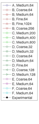
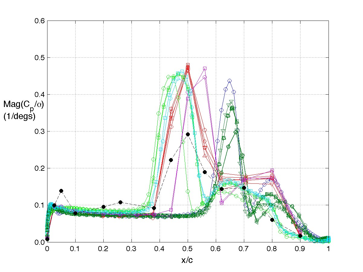
RSW, AePW Results: α = 2°, 10 Hz Forced Oscillation Results
Mach 0.825, Rec = 4M, Test medium: R-12
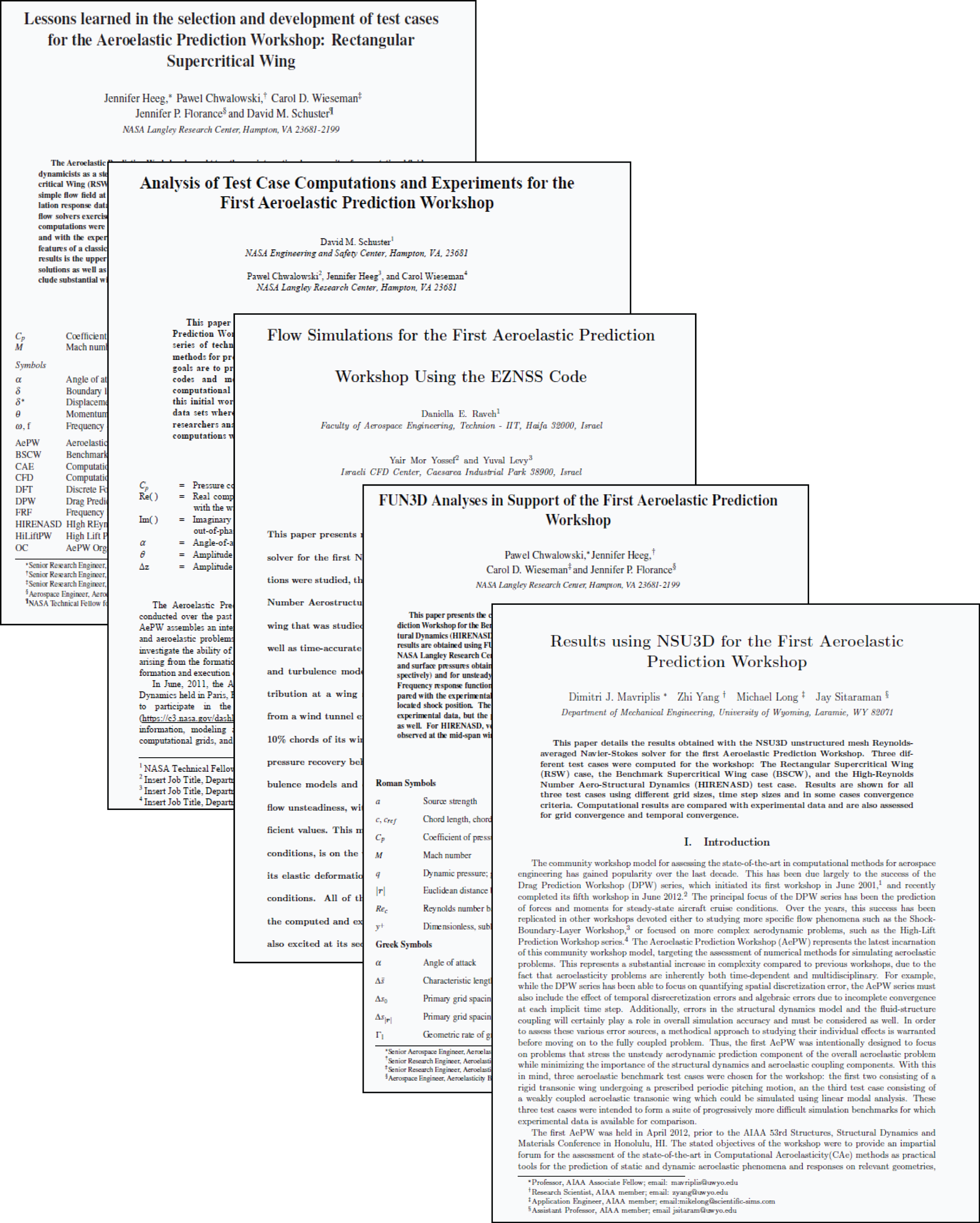
The RSW was oscillated in a pitching motion at 10 Hz. The results shown on this page are for forced oscillations about a mean angle of attack condition of 2°. The legend or key for the plots is shown at the left of the table. Note that the legend changes for each analysis/test condition. (i.e. it does not apply to the results on other pages.)
Frequency response functions
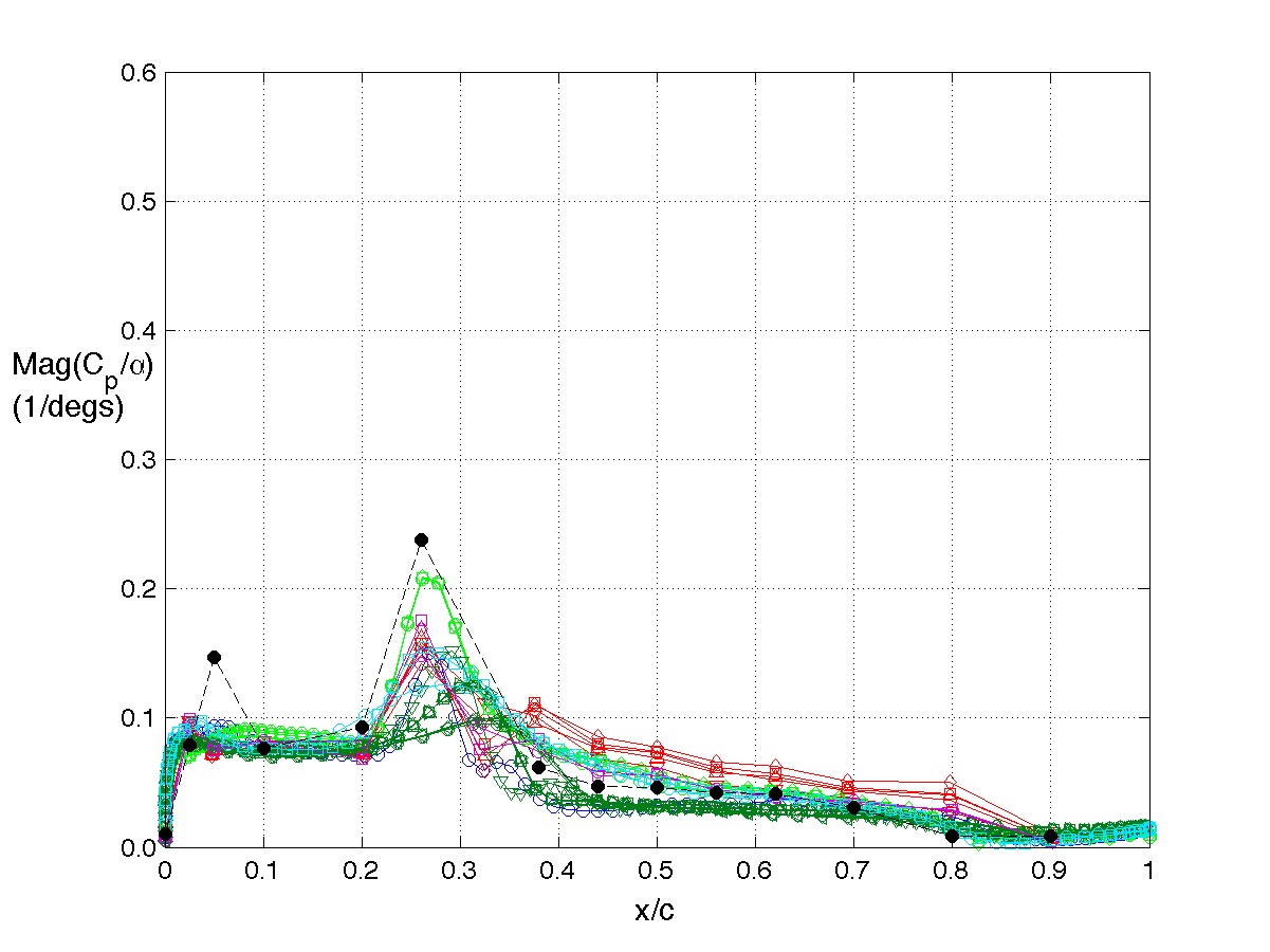
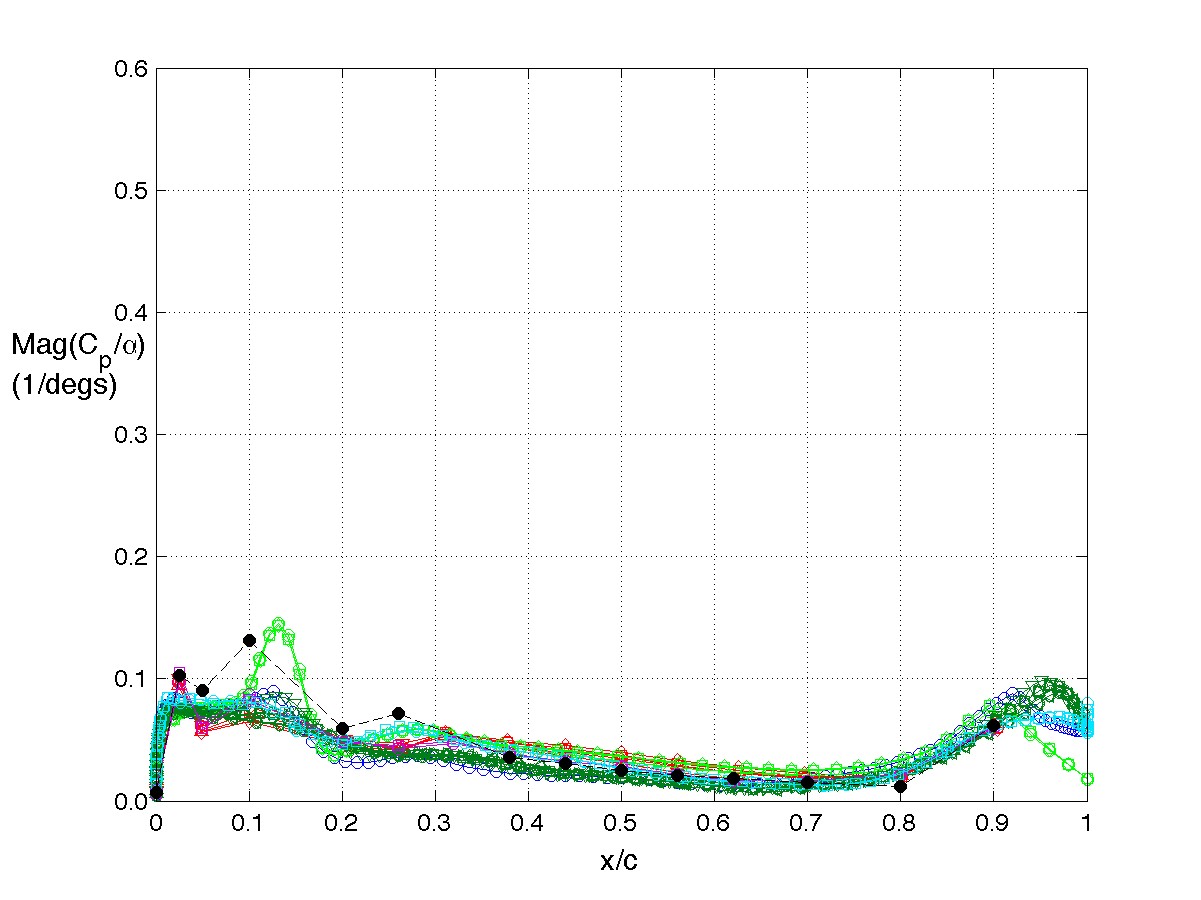
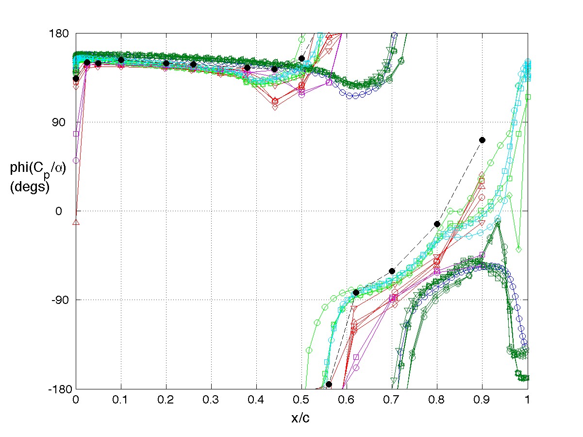
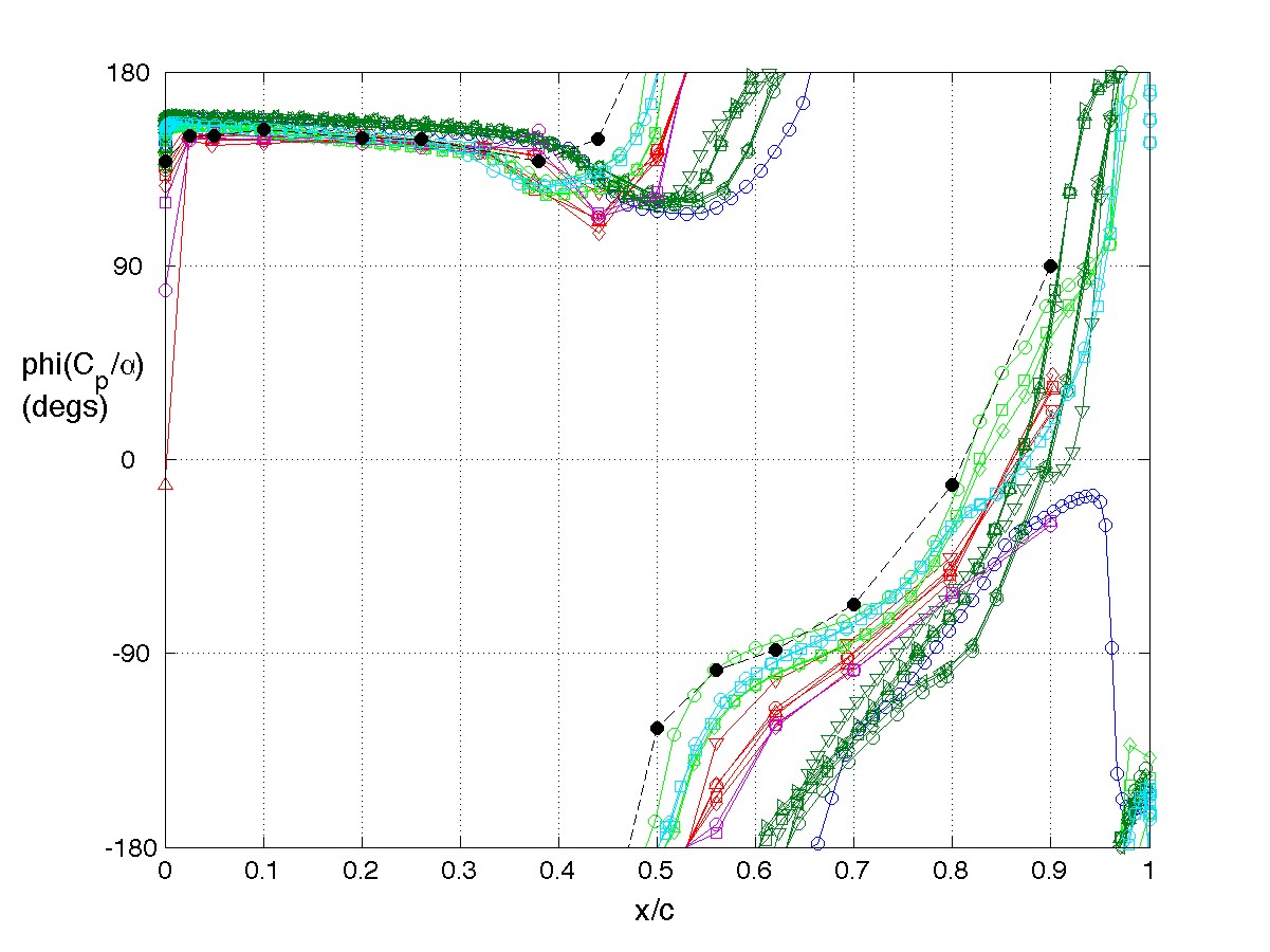
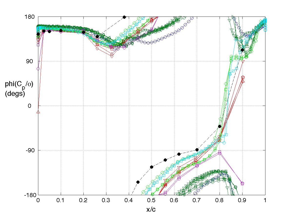
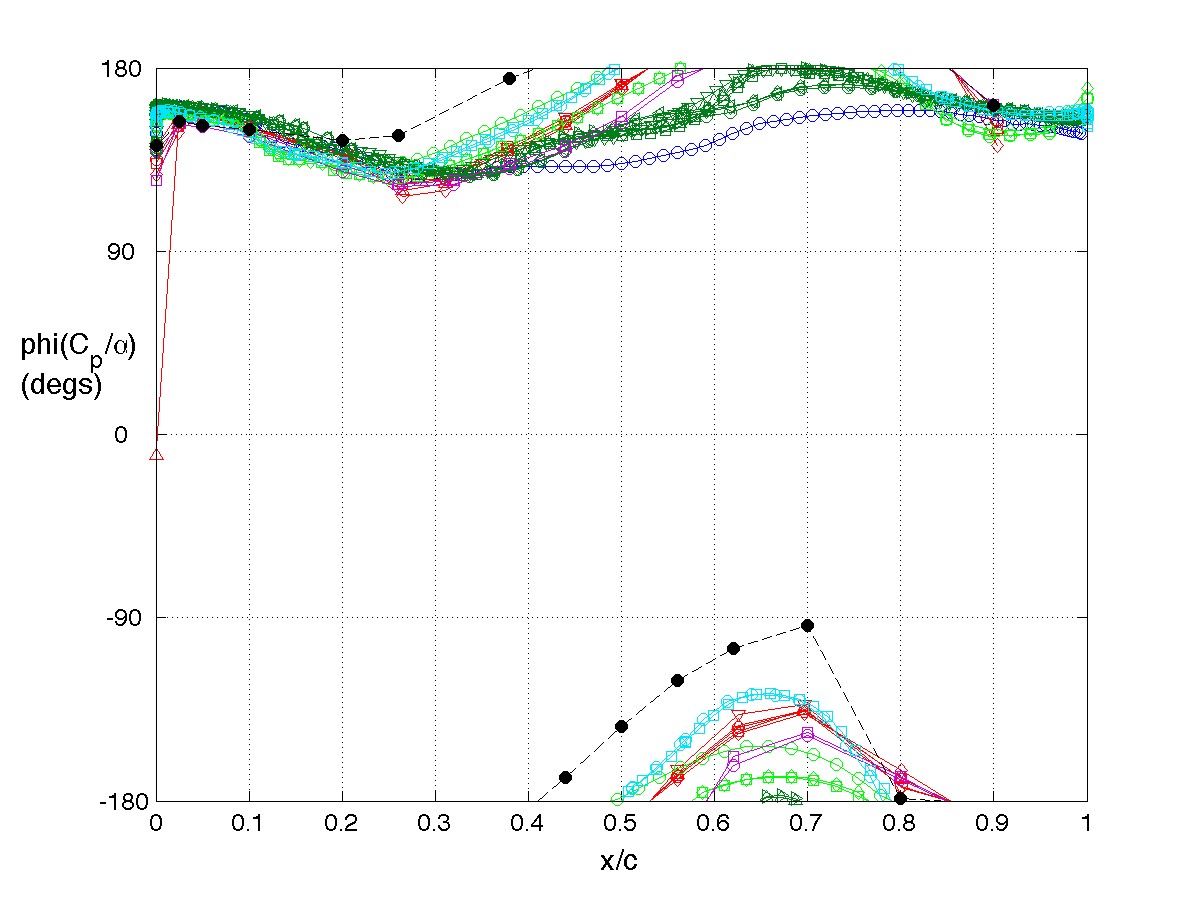
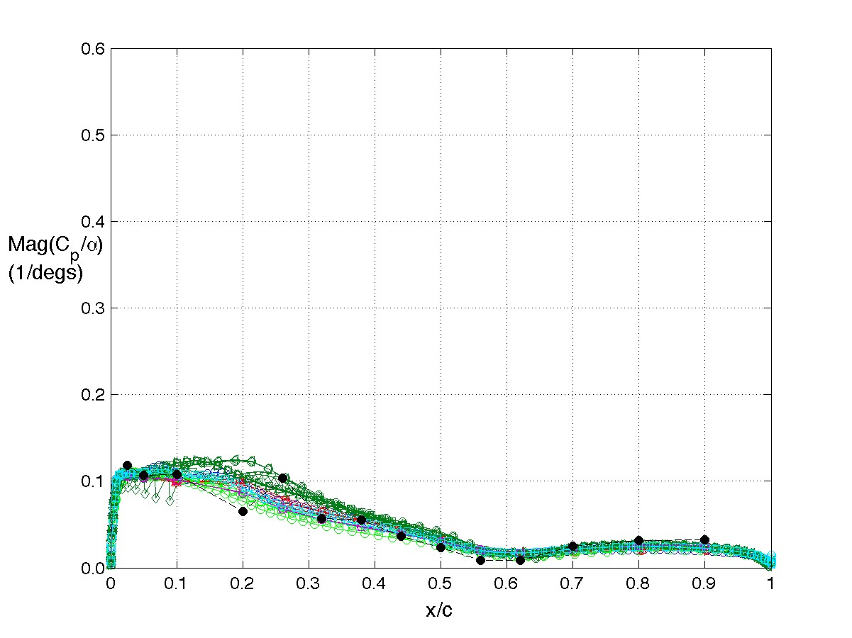
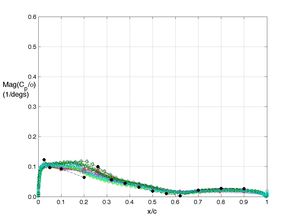
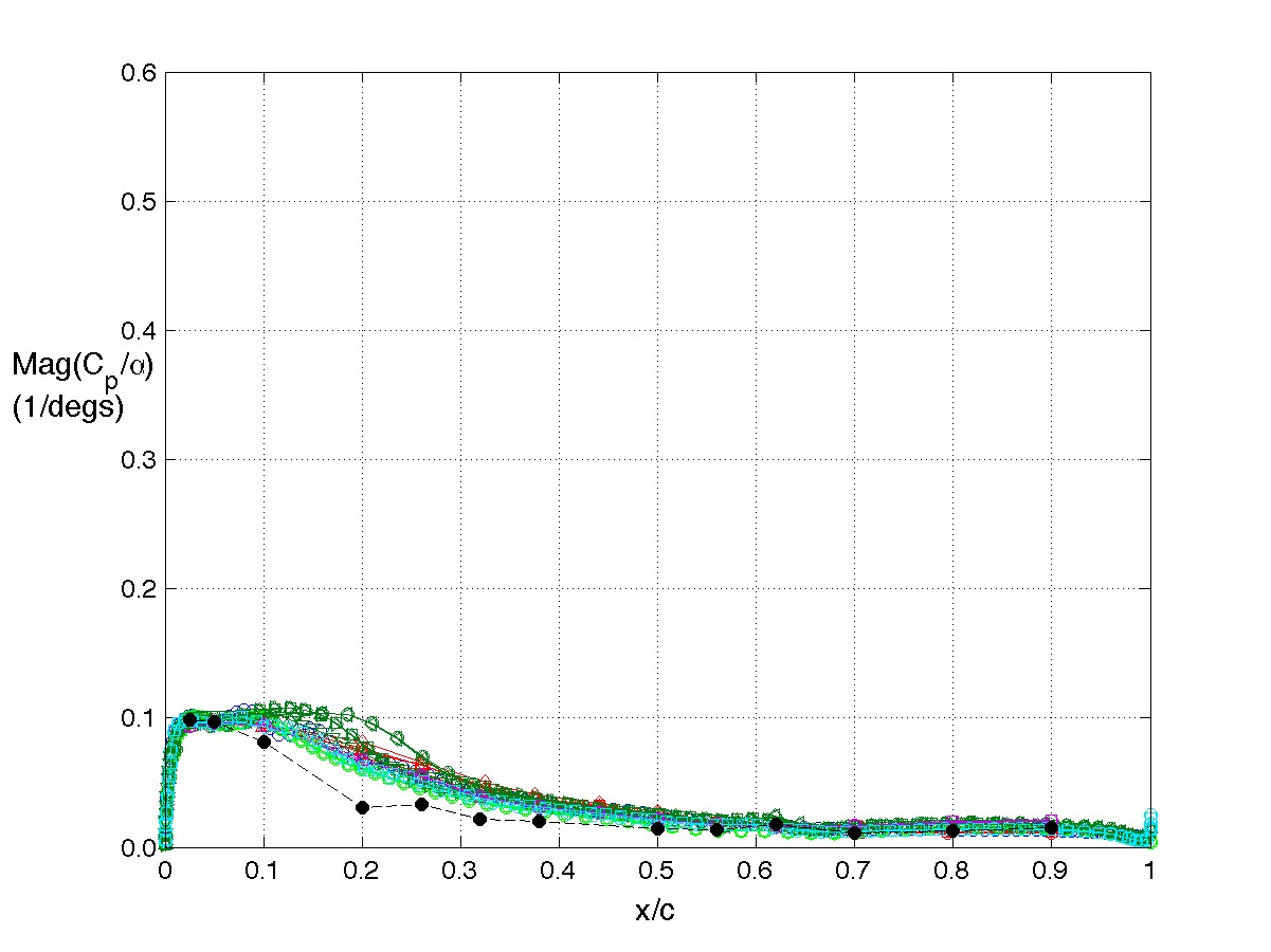
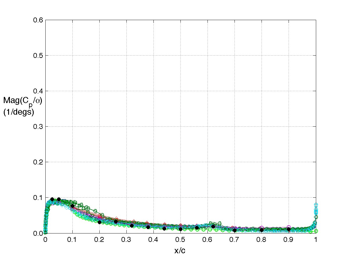
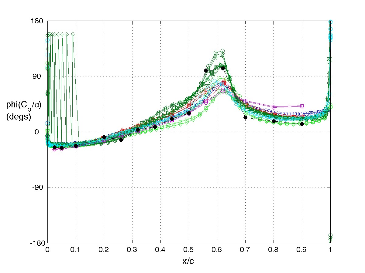
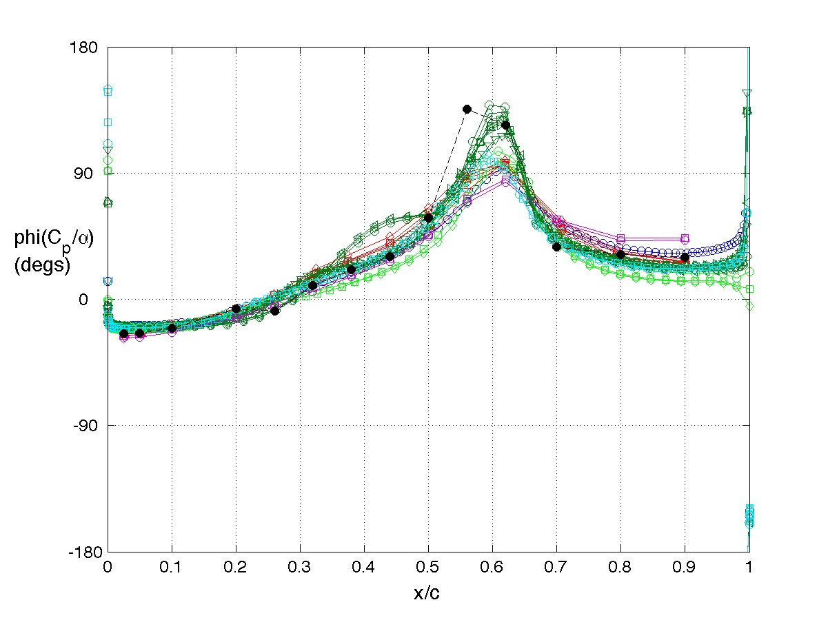
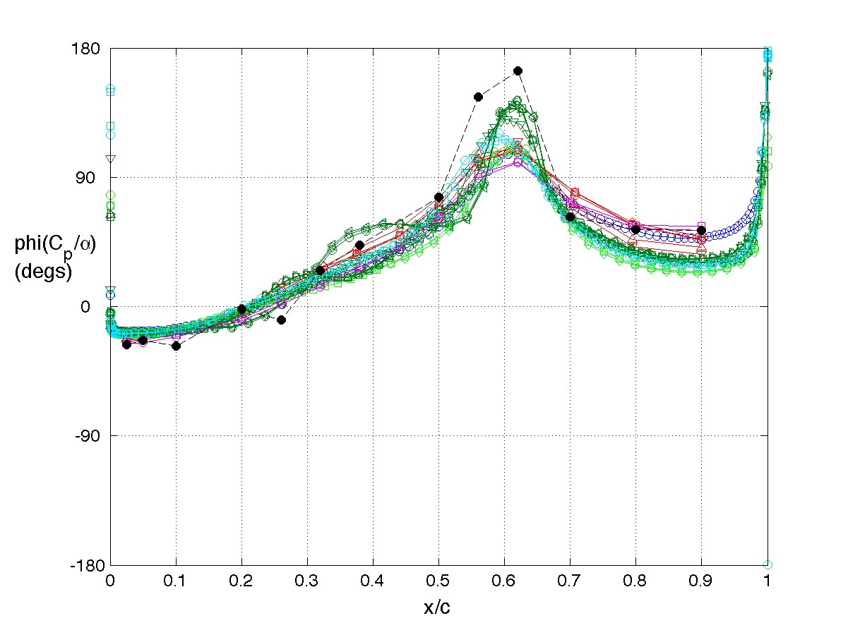
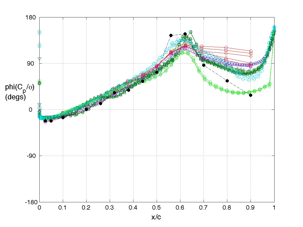
The principal comparison quantities generated from post-processing the computational outputs are the frequency response functions (FRFs) of the pressure coefficients due to the pitch angle. This data is presented at only the forcing frequency (that is, a single frequency point from the traditional FRF horizontal axis). The horizontal axis shows the normalized chord location of each of the pressure sensors and/or grid points.
The FRFs are presented below in terms of Magnitude & Phase components (i.e. the FRFs are shown in polar coordinates).
|
|
Time Convergence, lift coefficient
The integrated loads were computed by each analyst. However, there was confusion over the integration area and the normalizing constants. This confusion is likely responsible for the scatter seen in these results, rather than something inherent in the simulations. Here, the lift coefficient is actually the magnitude of the FRF of the lift coefficient due to angle of attack.Plotting vs time step. Note that on the plot, the black-filled symbols are fine grid solutions; the grey-filled symbols are medium grid solutions; the white-filled symbols are coarse-grid solutions.
-
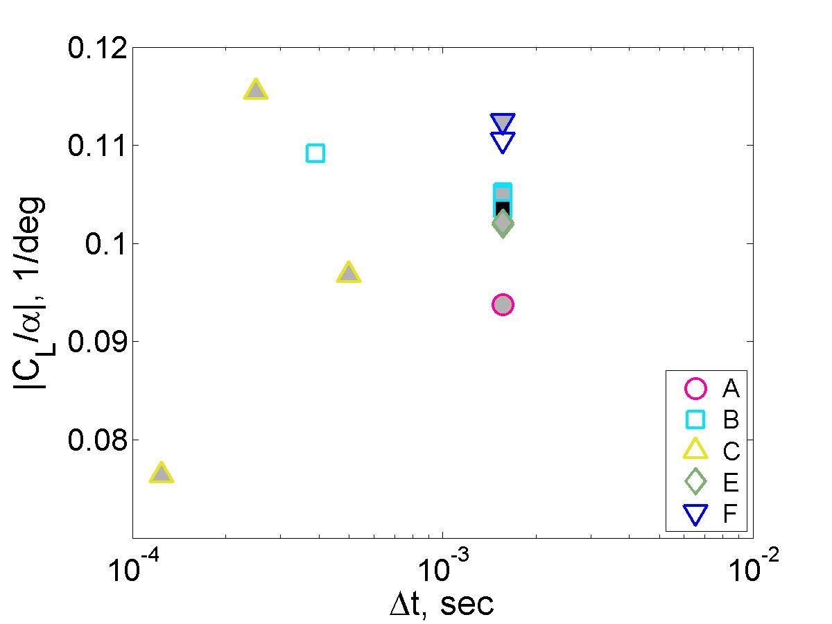
FRF Magnitude(Lift Coefficient due to angle of attack) vs Time step size
-
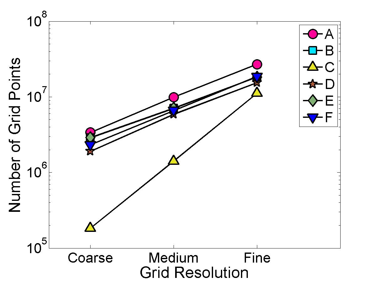
Grid Sizes used
Time History Comparisons
Time history information was requested from the analysts for their medium grid results at a few select sensor (grid point) locations. A forward station was specified and then the analysts were asked to select the location that they thought best represented the shock location. The pressure coefficients at these two locations are shown below. The times have been shifted such that the time histories line up as well as possible, so no phase information should be interpreted from these plots.Plotting vs time step.
-

Time histories, at a specified station intended to be ahead of the shock
-
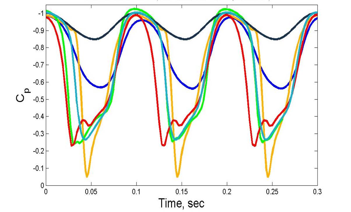
Time histories, at the analyst-chosen shock location