Forced Oscillation Results
Time-accurate simulations were performed, oscillating the wing rigidly through 1° amplitude oscillations of pitch, relative to the mean angle of attack, α = 2°. Two frequencies of oscillation were used for the RSW configuration: 10 & 20 Hz.
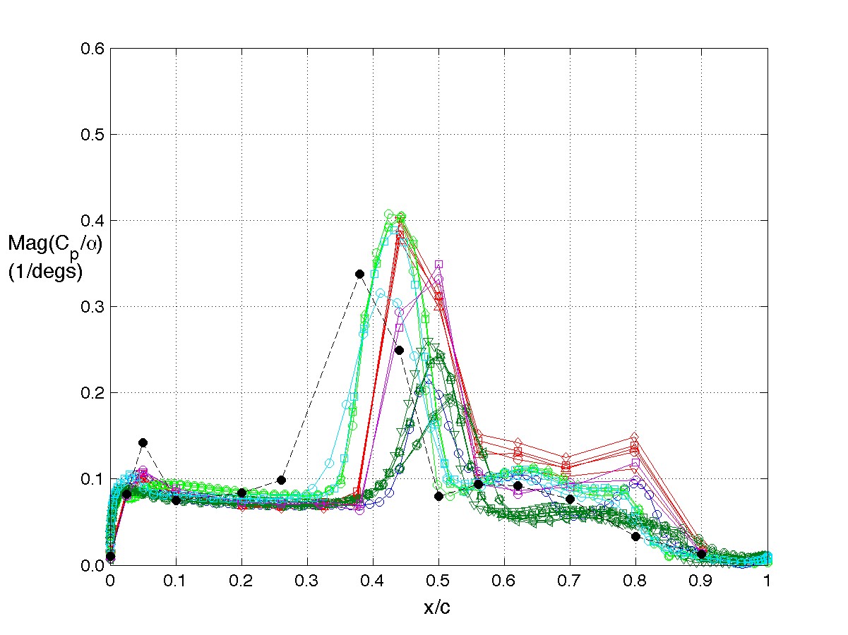
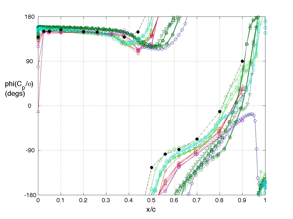
The principal comparison quantities generated from post-processing the computational outputs are the Frequency Response Functions (FRFs) of the pressure coefficients due to the pitch angle. The FRFs were computed and compared at only the frequencies of the forced oscillations. They are plotted as functions of non-dimensional chord location, x÷c. FRFs can be shown in either rectangular coordinates (Real & Imaginary components) or in polar coordinates (Magnitude & Phase).
The example plots shown on this page correspond to the response at span station 2, η= 0.59, upper surface pressure coefficient responses at 10 Hz. They are shown as Magnitude and Phase here.
AePW Database Files
Computational results...
submitted to the AePW were assembled into databases in MATLAB data structures. Files containing those databases for each data set can be accessed here.- Unforced system ("steady"), α = 2°
- Forced oscillation ("unsteady"), α = 2°, 10 Hz oscillation
- Forced oscillation ("unsteady"), α = 2°, 20 Hz oscillation
- Unforced system ("steady"), α = 4°
Corresponding experimental databases...
used for comparison for the AePW are also assembled into databases in MATLAB data structures. Files containing those databases for each data set can be accessed here.Unforced System ("steady") Results
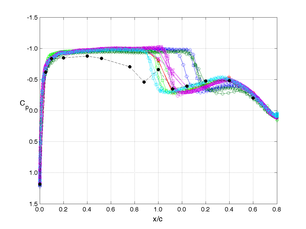
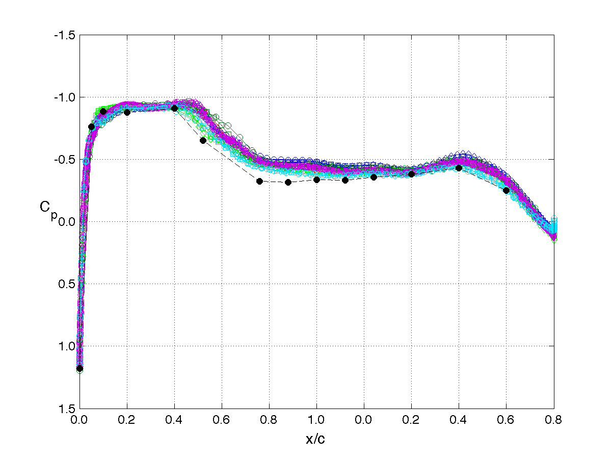
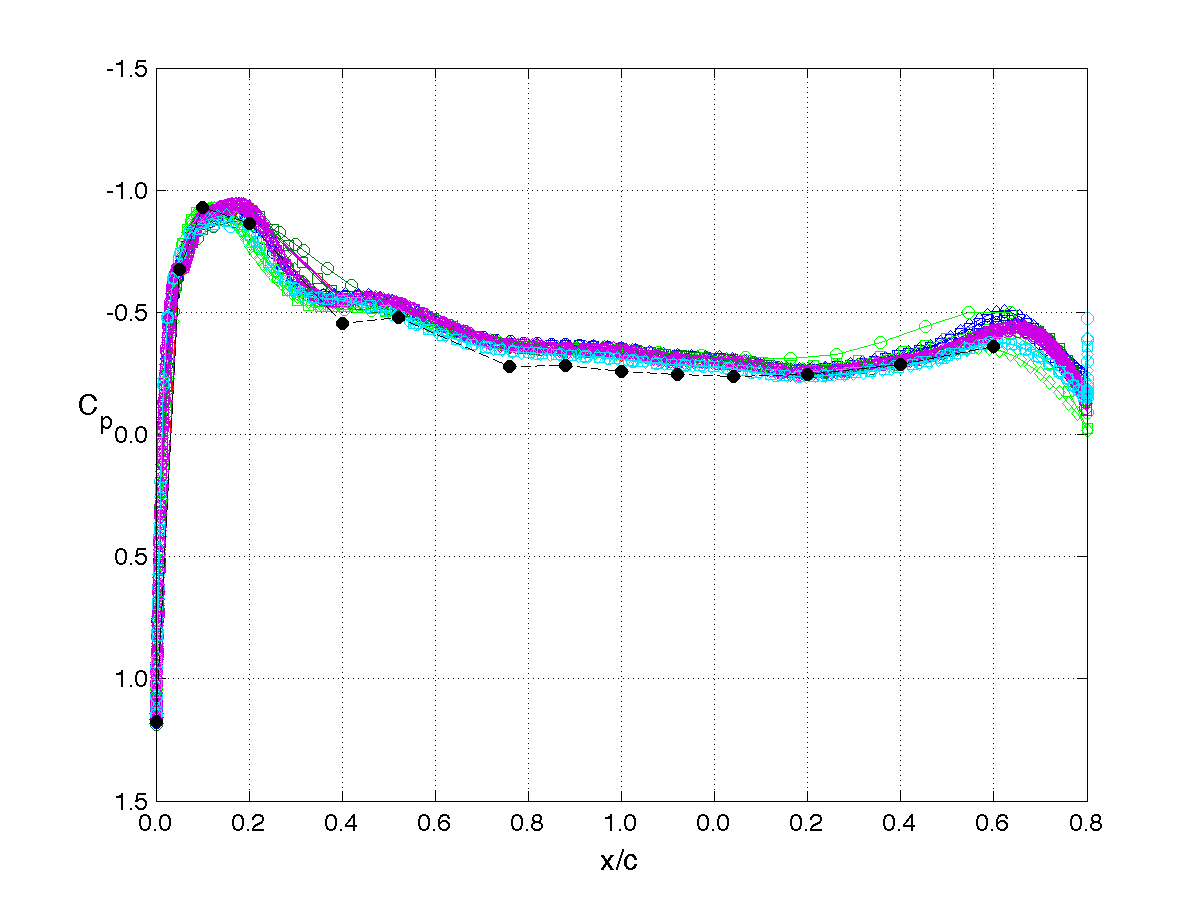
The unforced system is often referred to as the "steady" or "static" results. For AePW, most analysis teams analyzed the unforced system using a steady-state solution instead of a time-accurate solution. The analysis conditions for the unforced system correspond to the mean angle of attack condition for the forced oscillation case, 2°, and a second test condition at 4°.
The principal comparison quantities generated from post-processing the computational outputs are the pressure coefficient distributions. Other quantities calculated include the integrated force (lift & drag) and moment (pitching moment) coefficients.
The example plots shown on this page correspond to the upper pressure distributions at each of the 4 span stations.
-
Station 1, η= 0.309
-
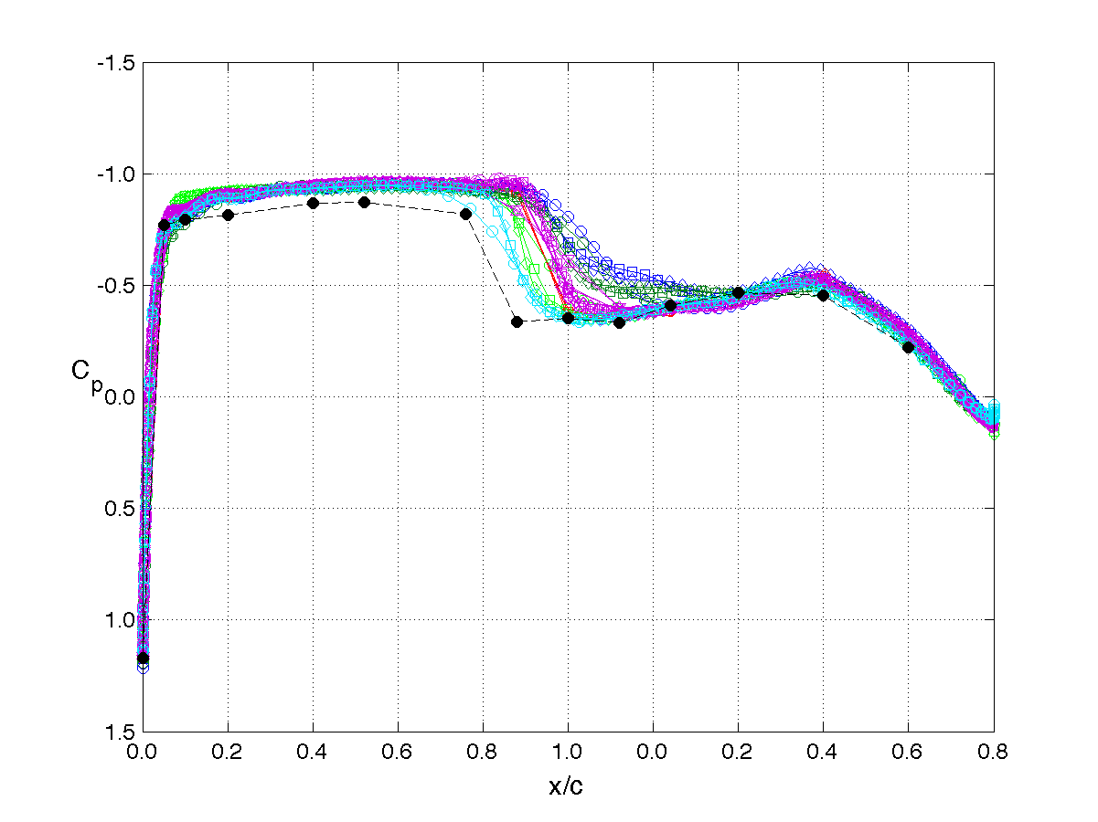
Station 2, η= 0.588
-
Station 3, η= 0.809
-
Station 4, η= 0.951
Computation Descriptions
-
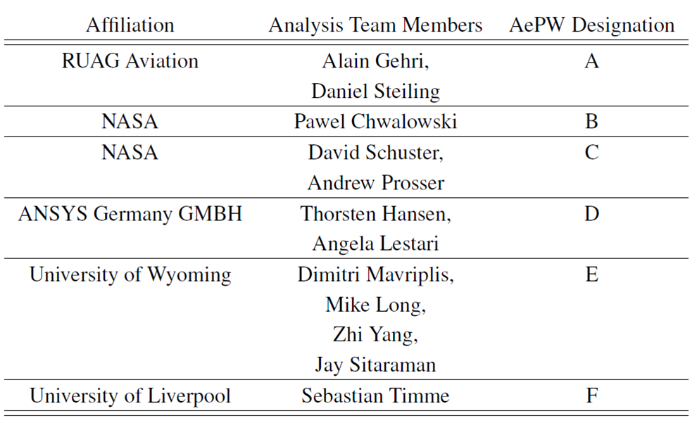
Analysis Teams
-

Flow Solvers
-
Analysis Teams
Flow solvers used by each team
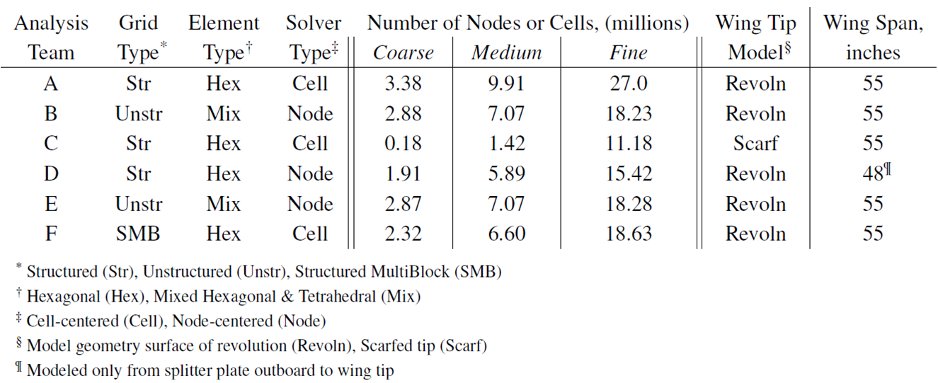
Grids used by each team
Influence of Simulation Options?
A few example plots are shown here.
-
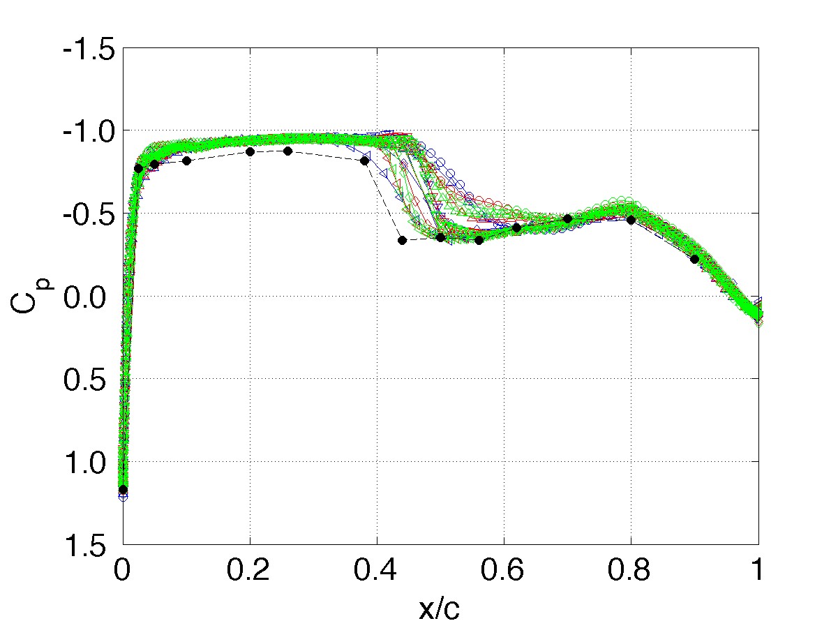
Grid Resolution: Unforced system response, α=2° Station 2, η= 0.588
-
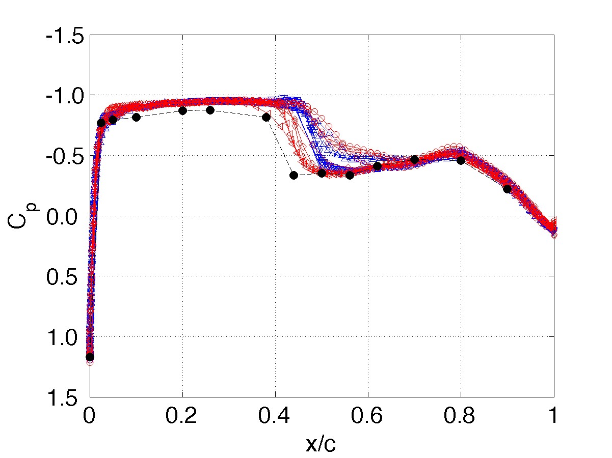
Solver Type: Unforced system response, α=2° Station 2, η= 0.588
-
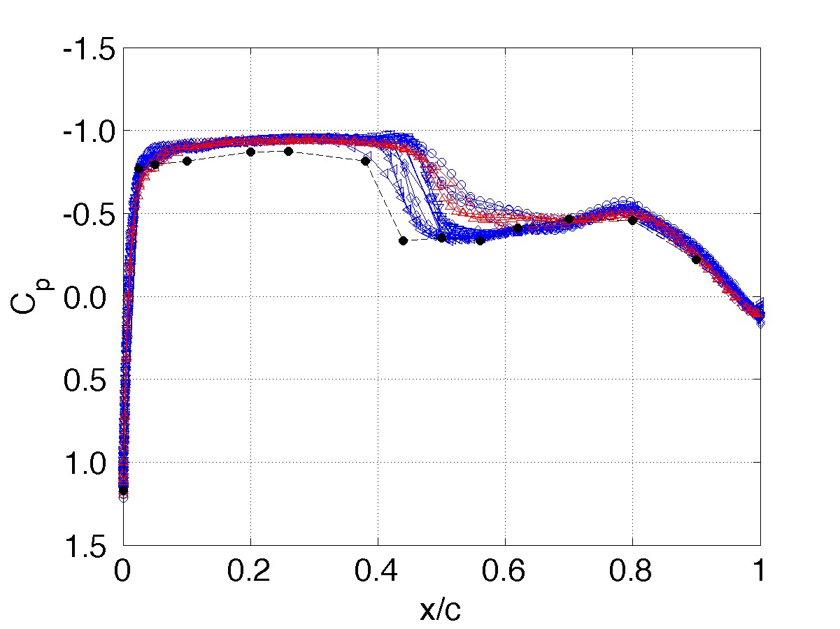
Turbulence Model: Unforced system response, α=2° Station 2, η= 0.588
-
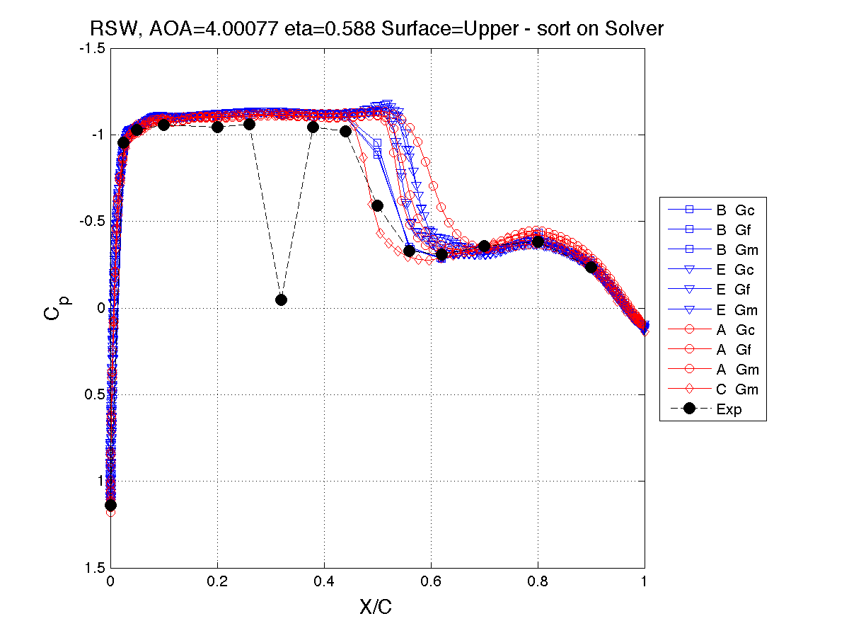
Solver Type: Unforced system response, α=4° Station 2, η= 0.588
-
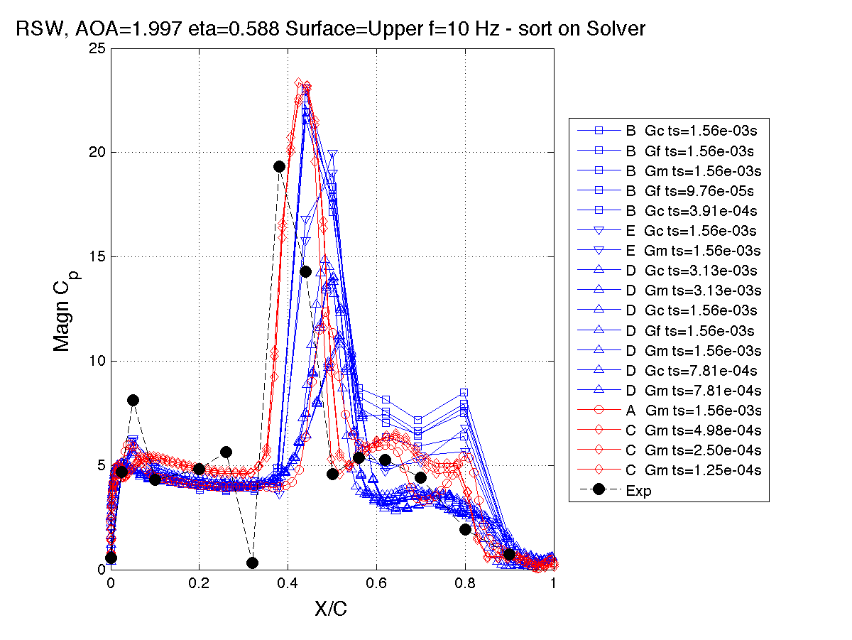
Solver Type: FRF Magnitude, 10 Hz, Station 2, η= 0.588
-
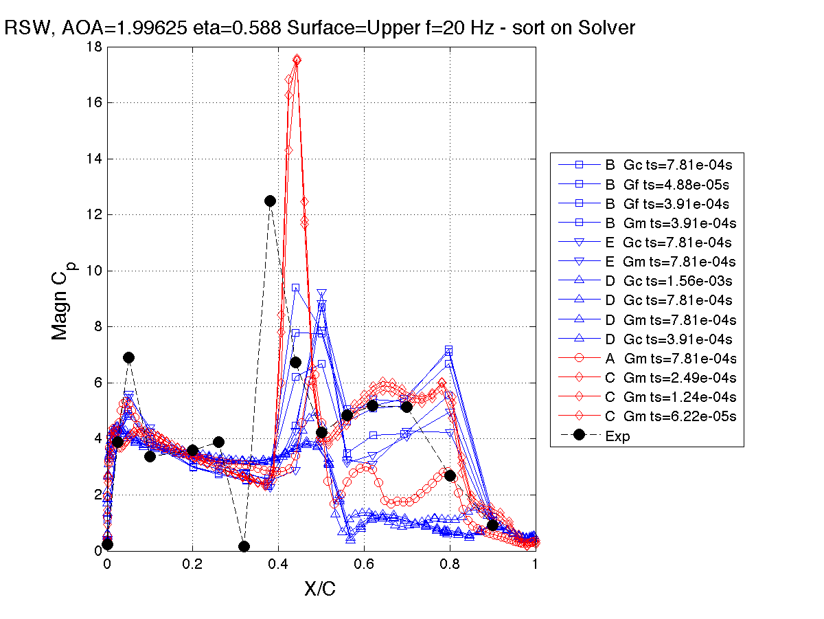
Solver Type: FRF Magnitude, 20 Hz, Station 2, η= 0.588
Publications and Presentations
Lessons learned in the selection and development of test cases for the Aeroelastic Prediction Workshop: Rectangular Supercritical Wing A summary paper including analysis of the experimental data and comparison with the computational results was presented at the 2013 AIAA Aerospace Sciences Meeting in Grapevine Texas. and the accompanying Presentation slides.
Geometrical and Properties of a Rectangular Supercritical Wing Oscillated in Pitch for Measurement of Unsteady Transonic Pressure Distributions; Ricketts, Watson, Sandford and Seidel - Nov 1983 (Ricketts)
AIAA-JA_vol21_no8.pdfTransonic Pressure Distributions on a Rectangular Supercritical Wing Oscillating in Pitch; Ricketts, Sandford, Seidel, Watson, Journal of Aircraft, Vol 21 No 8, 1983
1999046117.pdfComputational Test Cases - early RSW (Ricketts - in RTO publicaton) - Complete results are in NASA TM 85765 - Subsonic and Transonic Unsteady- and Steady-Pressure Measurements on a Rectangular Supercritical Wing Oscillated in Pitch by Ricketts, Sandford, Watson